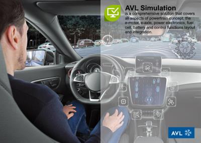
AVL Simulation Suite 2022 R2 | 9.2 Gb
Product:AVL Simulation Suite
Version:2022 R2 Build 248
Supported Architectures:x64
Website Home Page :www.avl.com
Languages Supported:english
System Requirements:Windows *
Size:9.2 Gb
The software developer Advanced Simulation Technologies (AST) is pleased to announce the availability of AVL Simulation Suite 2022 R2 is a comprehensive solution that covers all aspects of powertrain concept, the e-motor, e-axle, power electronics, fuel cell, battery and control functions layout and integration.
Release 2022 R2
We are pleased to announce the latest software releases for the following solutions:
Updates and improvements to AVL's simulation solution
Analyze Batteries Electrochemically
Release 2022 R2 of AVL CRUISE M makes the electrochemical simulation of batteries easier and more accurate. For this purpose, two major enhancements have been made.
CRUISE M now provides you with a tailored EIS Parameterization Wizard that simplifies the process of finding the electrode diffusion coefficient based on measured data. The "find the equivalent circuit" option starts the automatic search for the best fitting approach.
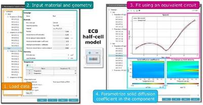
Figure 1: Electrochemical impedance spectroscopy wizard (EISW)
Double layer effects are now considered. The double layer induces an electrical field that is capable of storing and releasing charge in much less time than the intercalation process of lithium ions, like in a capacitor. Such high frequency responses are covered as part of the existing electrochemical battery at four different positions. First, at the electrode-electrolyte interface of the cathode and anode, and second, at the interfaces between the current collector plates and the adjacent electrodes.
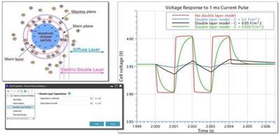
Figure 2: Double layer model concept and simulation results
Cylindrical Battery Module Now Available
The module "component cylindrical cell" is the extension to the prismatic and pouch cells that are already available.
It allows you to define the cell arrangement, the housing configuration, the cooling type, the electrical connection pattern and all types of connection ports, as well at the measuring points for interaction with other components. The cells are modeled in 2D featuring different temperatures in radial direction and across their height. It supports both equivalent circuit models and Batemo cell models.
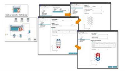
Figure 3: Battery module - cylindrical - parameterization workflow
Solution: Mechanical stresses on battery
In addition to the thermal and electrical states in batteries, it is important to consider their mechanical behavior during operation. We take this into account with two functional enhancements.
Tilting of pouch cells in battery modules
Pouch cells are usually connected to the bottom of the enclosure via a thermal paste. The fact that cells are fixed at the bottom and the other sides are more flexible to move also impacts the expansion/contraction of cells and the mechanical stresses that build up. This version of CRUISE M offers the possibility to model cell tilting.
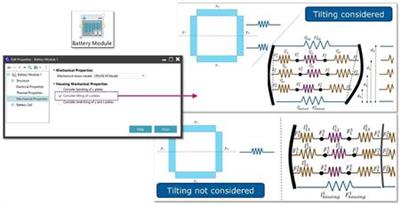
Figure 4: Battery module: Tilting of battery cells
A new interface is available should you need to integrate custom model extension into existing CRUISE M models. The interface allows you to integrate your user-defined sub model without having to sacrifice the comfort of the overall solution.
The Battery-Module has been extended by a dedicated interface for mechanical models. This allows the custom models to describe all mechanical aspects of the module's housing that react to expanding and contracting battery cells.
The model needs to be given as FMU complying to a dedicated interface specification defined by CRUISE M.
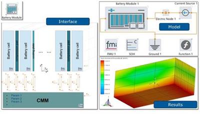
Figure 5: Battery module: Integration concept for custom mechanical models
Solution: Battery Safety Analysis
Easy simulation of battery thermal behavior in the event of thermal runaway.
Another new feature of the Battery Module component allows you to study the propagation of heat through a module assembled from cells, cooling plates, and pressure pads. The input is the heat released by the cell during thermal runaway. You can determine this information using abuse tests on a single cell and the Compose app. Together with the actual cell energy and a trigger temperature, this input is sufficient to model the thermal history of a single cell. You can view the local temperature rise in a cell and the spillover to neighboring cells, as well as the propagation across the entire module.
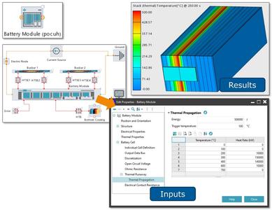
Figure 6: 3D Battery module: Temperature distribution through structure
Solid Particle Release:
AVL FIRE M is now able to simulate the exertion of solid particles during battery cell venting. The particles are modelled using a Lagrangian description of particle motion. Coupling of energy, momentum and turbulence exchange with the surrounding gas phase is taken into account. Specific sub models are used for the drag law and evaporation.
Methodology development has shown that consideration of these particles can provide additional insights into the occurring risks posed by particles, as shown in Figure 7.
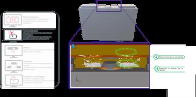
Figure 7: Solid particles during the battery cell venting event. Particles melt the golden, meltable parts and pose an additional threat due their ignition energy
.
Updates and improvements to AVL's simulation solution
Introduction of AVL EXCITE M
With Release 2022 R2 of AVL EXCITE M, we are launching a new generation of our multi-body dynamics software solution for powertrain analysis.
The first step was the migration of EXCITE for e-axle. By integrating a new IC motor assembly, you can now simulate both e-drive units and hybrid configurations with IC engines. Improved load and signal processing capabilities are available for more accurate simulation of transient operating conditions.
In a second step, EXCITE Power Unit will also be migrated to enable the modeling, simulation and evaluation of structural dynamics, NVH and durability of any powertrain configuration in a single interface.
IC-Engine Assembly
EXCITE M supports the modelling of common configurations of internal combustion engines by providing an IC-Engine Assembly element.
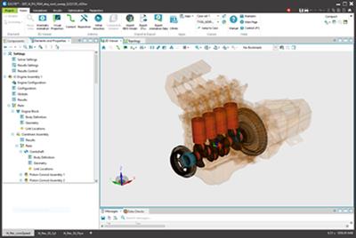
Figure 1: IC-engine assembly of an I4 engine
The element allows you to specify:
- IC-engine configuration (such as number of cylinders, their arrangement, several basic dimensions, and firing order)
- Model fidelity (such as usage of axial bearings, connection representation to be used for piston/liner guides and enabled degrees of freedom for certain components)
- Global geometry (such as bore and bearing dimensions) and cylinder pressure load
Based on the above inputs, the basic IC-engine model is automatically built. All parts of the model (bodies and joints, partly structured in sub-assemblies) are configured. Once the automatic setup of the base model is complete, the user can adjust certain parts or components to fit them to specific modeling and/or geometrical requirements. This could be related to the exact positioning of a pulley or flywheel on a crankshaft, for instance, or concern details regarding the node distribution used to connect the parts of the system.
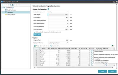
Figure 2: Adjustment of components on a crankshaft
In addition, the IC-Engine Assembly generates all sub-parts (link location types and positions) to enable the easy search of connection nodes or node sets. The condensation of FE models for flexible bodies is supported by the Component Modeler and enables the easy application of all used joints to the corresponding nodes on the connected bodies.
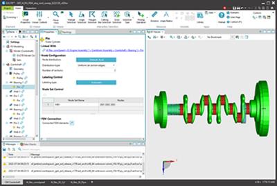
Figure 3: Component modeler view for a crankshaft model
Working with existing condensed body representations is also possible. In this case, you can explicitly correlate the nodes and node sets in the FE model to the joint created in the IC-Engine Assembly. This step is supported by the select and search capabilities in the GUI.
Cylinder Pressure Load
A special cylinder pressure load definition has been introduced together with the IC-Engine Assembly to support the modeling of systems for transient dynamic analysis.
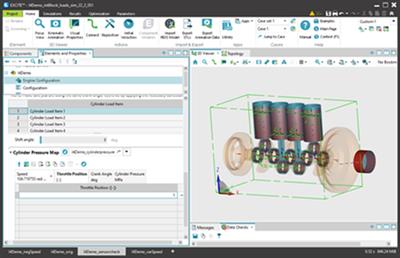
Figure 4: Cylinder pressure specification
Cylinder pressure can be specified in a map as crank-angle-related pressure dependent on engine speed and throttle signal. The cylinder pressure is specified for a discrete number of operating points (engine speed or throttle position combinations). The reference quantities for the cylinder pressure load evaluation are defined with the load properties. Sensor elements can be used to determine the actual state of these quantities during the simulation.
- Speed reference can be set to a user-defined constant value or by using a sensor element to pick up an angular velocity of a body or a relative velocity between two bodies.
- Crank angle reference can use the same reference motion for all cylinders, or you can select reference motions from different sensors for the individual cylinders.
- Throttle demand can currently be defined by a user-defined constant value or by a table vs. time or reference angle.
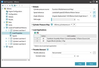
Figure 5: Reference quantities for cylinder pressure load assignment
The correct transfer from specified cylinder pressure to appropriate load forces on the model components is defined in the Load Application panel. Two ways of load assignment are supported:
- Application of loads to nodes: Here, the type of the load signal can be defined (pressure, force, moment) and the distribution of the defined load to the individually connected nodes must be specified. For standard modeling cases, all required settings are done automatically based on the given IC-Engine Assembly data.
- Alternatively, the loads can be distributed to the body's connected nodes using load case vectors, prepared with the FE model of the body.
Signal Network
Several new elements to model simple control system functionality are provided to be able to influence and control system behavior such as cylinder pressure application (e.g. via changing the throttle position) or performing switching actions in a drive system (e.g. actuating a clutch).
In addition, the possibility of integrating C-code in the form of so-called compiled functions allows basic control functions (e.g. a PI controller) to be incorporated. Co-simulation with external tools is no longer necessary.
- Another innovation concerns signals and control. A first set of components is now offered to you in the graphical front-end of EXCITE M): Load Applicator and Load Item Cylinder Pressure: Facilitate load application at body nodes (like pressure, force and moment) based on the specified input-signals.
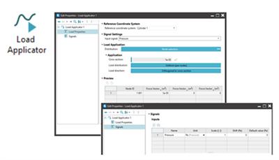
Figure 6: Load applicator component to convert signals into pressure, force, moment

Figure 7: Cylinder pressure load map utilizing signal input for crank angle, speed and throttle position
-Elasto-Plastic Clutch Joint (EPCL) and Table Force/Moment Joint (FTAB):In order to model and actuate switching elements such as friction clutches, simple synchronizer units or dog clutches, the existing joint functionality has been extended. The extension includes the joint properties clamping force, stiffness/damping. These can now be set and scaled via input signals.
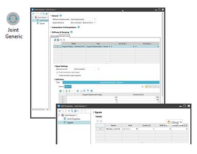
Figure 8: Force/moment joint (FTAB) force/moment application and scaled by table

Figure 9: Elasto-plastic friction clutch (EPCL): Clutch actuation by clamping force depending on closing ratio signal
-Motion Sensor:Measuring the rotary speed of a shaft/crankshaft at a specific node position relative to a housing or engine block is complex. This new component allows you to sense and process relative translational and rotational motions between the nodes of two bodies. Moreover, it provides you with basic functions for the conversion of 3D vector readings into single signals such as vector norm or scalar projection.
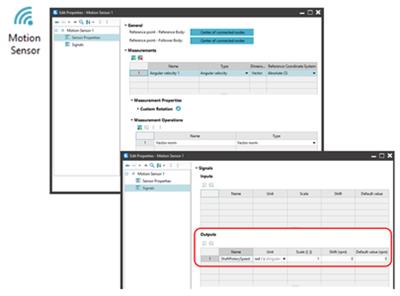
Figure 10: Motion sensor for the measurement of relative translational/rotational quantities between body nodes
-Force/Moment Sensor:The existing Table Force/Moment Joint (FTAB) has been extended to perform basic force/moment measurement tasks. For each of the different FTAB options, the resulting force/moment can be accessed via an output signal provided by the joint.
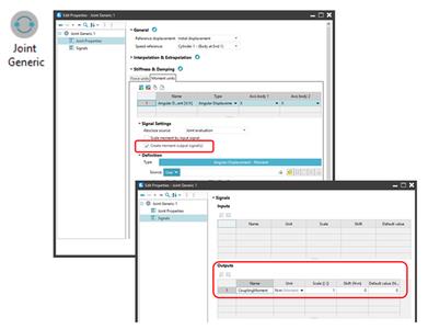
Figure 11: Force/moment sensor facilitated by Table Force/Moment Joint (FTAB)
-Function:The user can take any input and output signal of EXCITE model and use them in code that will perform a certain function in that model. Compilation of the C-code and link to EXCITE solver happens automatically and does not require any user action. This enables the user to significantly extend the functionality of EXCITE to fulfill his or her specific requirements.
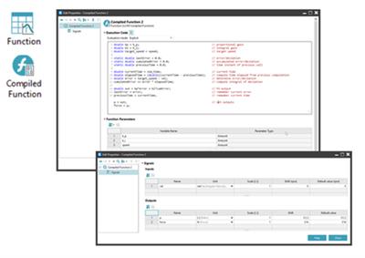
Figure 12: Simple speed-controller (PI) realized by a compiled function
Model.CONNECT Interface
It is now possible to connect EXCITE M with Model.CONNECT. This can be achieved using the new components. Any number of Model.CONNECT interfacing components can be arbitrarily added in the EXCITE M model. The Model.CONNECT components are part of the signal network in EXCITE M. This means that you have the possibility to define input and output signals for all EXCITE M quantities to be exchanged.
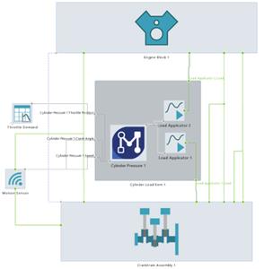
Figure 13: Example of connecting the Model.CONNECT component to bodies/sensors
Thermodynamic Coupling with Model.CONNECT
To support transient operating conditions such as start/stop simulations of hybrid engines, the Model.CONNECT interface is used to enable the thermodynamic coupling of EXCITE M with Model.CONNECT.
This is realized by adding a new option in the Load Item Cylinder Pressure to set the cylinder pressure source to Model.CONNECT. By selecting this option, a Model.CONNECT component is automatically inserted into the EXCITE M model and all required input and output signals are created and connected automatically.
Through the co-simulation with Model.CONNECT, the cylinder pressure can be calculated by the desired thermodynamic tool (e.g. CRUISE M). The pressure data will then be sent to EXCITE M where the pressure is transformed to a force and applied to the corresponding bodies by the Load Item (see the figure below).
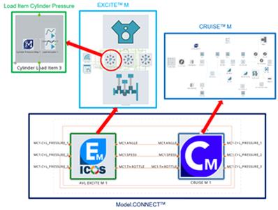
Figure 14: Three-cylinder engine model in AVL EXCITE M receiving cylinder pressure load from a thermodynamic model in
AVL CRUISE M via Model.CONNECT Co-Simulation
Electric Motor Joint Extensions
So far, EXCITE has offered joint types for acoustic analysis up to high frequencies of 20 kHz for all machine types. Now additional joint types and current controllers have been introduced to enable analysis of low-frequency problems in traction motor and hybrid applications.
EXCITE M offers following approach for electric motor joint:
- Map based (imported pre-calculated forces and moments) - available for all e-motor types with radial flux
- Parameter based (linear fundamental wave model) - available for PMSM (permanent-magnet synchronous motors), EESM (externally excited synchronous motors), SCIM (squirrel-cage induction motors) and SYRM (synchronous reluctance motors)
- File based - available for PMSM
. Saturated fundamental wave model - files for current dependent inductances and Permanent Magnet flux linkage
. MFC (Magnetic Field Computation) - files for phase-to-phase flux linkages and torque / stator tooth force / tooth axial moment
.. 'Axial-Axial': Rotor axis nodes coupled to stator axis nodes (with or without consideration of rotor eccentricity)
.. 'Axial-Circumferential': Rotor axis nodes coupled to stator teeth nodes (with or without consideration of rotor eccentricity)
New control systems have been introduced for the EESM and SCIM that reflect state-of-the-art current control for traction applications in motor or recuperation mode.
Updates and improvements to AVL's simulation solution
Introducing the next generation of AVL EXCITE M
With Release 2022 R2 of AVL EXCITE M, we are launching a new generation of our multi-body dynamics software solution for powertrain analysis.
The first step was the migration of EXCITE for e-axle. By integrating a new IC motor assembly, you can now simulate both e-drive units and hybrid configurations with IC engines. Improved load and signal processing capabilities are available for more accurate simulation of transient operating conditions.
In a second step, EXCITE Power Unit will also be migrated to enable the modeling, simulation and evaluation of structural dynamics, NVH and durability of any powertrain configuration in a single interface.
Frequency Domain Solution (FDS) for Transmission Systems
For application scenarios such as standard gearbox-NVH, optimization/DoE tasks and others EXCITE M offers you a faster solution: the new frequency domain solution (FDS). You can use FDS as an alternative to the well-known time domain solution (TDS) or as a supplement. The relevant sources for periodic excitation of e-axles are gear excitation forces. Analytical tooth contact analysis (TCA) is used to calculate these gear excitation forces.
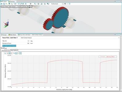
Figure 1: Analytical tooth contact analysis in gear joint's focus view
The solution provides results for all nodal body motion quantities (i.e., displacements / velocities / accelerations) over the analyzed frequencies.
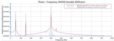
Figure 2: Body nodal angular velocity - comparison between FDS and TDS
To display the results in other coordinate systems, the synthesis of the results in the angle/time domain is supported.
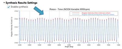
Figure 3: Result synthesis - comparison between FDS and TDS
In addition to chart-based representations, you now have the option to animate the 3D FDS results in two different ways:
- By body motion at single frequencies (including data recovery of nodal quantities)
- By synthesizing body results that represent the combination of the single frequencies to a time and angle equivalent signal
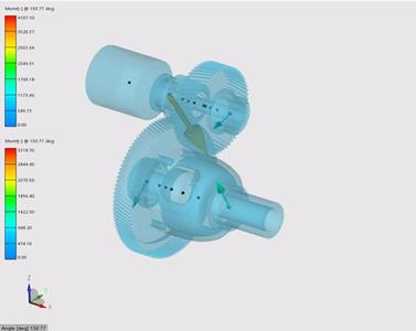
Figure 4: Animation of synthetized frequency domain body results in AVL IMPRESS M
Signal Network
Several new elements to model simple control system functionality are provided to be able to influence and control system behavior such as cylinder pressure application (e.g. via changing the throttle position) or performing switching actions in a drive system (e.g. actuating a clutch).
In addition, the possibility of integrating C-code in the form of so-called compiled functions allows basic control functions (e.g. a PI controller) to be incorporated. Co-simulation with external tools is no longer necessary.
- Another innovation concerns signals and control. A first set of components is now offered to you in the graphical front-end of EXCITE M): Load Applicator and Load Item Cylinder Pressure: Facilitate load application at body nodes (like pressure, force and moment) based on the specified input-signals.

Figure 5: Load applicator component to convert signals into pressure, force, moment

Figure 6: Cylinder pressure load map utilizing signal input for crank angle, speed and throttle position
-Elasto-Plastic Clutch Joint (EPCL) and Table Force/Moment Joint (FTAB):In order to model and actuate switching elements such as friction clutches, simple synchronizer units or dog clutches, the existing joint functionality has been extended. The extension includes the joint properties clamping force, stiffness/damping. These can now be set and scaled via input signals.

Figure 7: Force/moment joint (FTAB) force/moment application and scaled by table
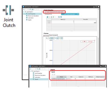
Figure 8: Elasto-plastic friction clutch (EPCL): Clutch actuation by clamping force depending on closing ratio signal
-Motion Sensor:Measuring the rotary speed of a shaft/crankshaft at a specific node position relative to a housing or engine block is complex. This new component allows you to sense and process relative translational and rotational motions between the nodes of two bodies. Moreover, it provides you with basic functions for the conversion of 3D vector readings into single signals such as vector norm or scalar projection.
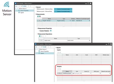
Figure 9: Motion sensor for the measurement of relative translational/rotational quantities between body nodes
-Force/Moment Sensor:The existing Table Force/Moment Joint (FTAB) has been extended to perform basic force/moment measurement tasks. For each of the different FTAB options, the resulting force/moment can be accessed via an output signal provided by the joint.

Figure 10: Force/moment sensor facilitated by Table Force/Moment Joint (FTAB)
-Function:The user can take any input and output signal of EXCITE model and use them in code that will perform a certain function in that model. Compilation of the C-code and link to EXCITE solver happens automatically and does not require any user action. This enables the user to significantly extend the functionality of EXCITE to fulfill his or her specific requirements.
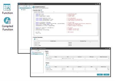
Figure 11: Simple speed-controller (PI) realized by a compiled function
Model.CONNECT Interface
It is now possible to connect EXCITE M with Model.CONNECT. This can be achieved using the new components. Any number of Model.CONNECT interfacing components can be arbitrarily added in the EXCITE M model. The Model.CONNECT components are part of the signal network in EXCITE M. This means that you have the possibility to define input and output signals for all EXCITE M quantities to be exchanged.

Figure 12: Example of connecting the Model.CONNECT component to bodies/sensors
Electric Motor Joint Extensions
So far, EXCITE has offered joint types for acoustic analysis up to high frequencies of 20 kHz for all machine types. Now additional joint types and current controllers have been introduced to enable analysis of low-frequency problems in traction motor and hybrid applications.
EXCITE M offers following approach for electric motor joint:
- Map based (imported pre-calculated forces and moments) - available for all e-motor types with radial flux
- Parameter based (linear fundamental wave model) - available for PMSM (permanent-magnet synchronous motors), EESM (externally excited synchronous motors), SCIM (squirrel-cage induction motors) and SYRM (synchronous reluctance motors)
- File based - available for PMSM
. Saturated fundamental wave model - files for current dependent inductances and Permanent Magnet flux linkage
. MFC (Magnetic Field Computation) - files for phase-to-phase flux linkages and torque / stator tooth force / tooth axial moment
.. 'Axial-Axial': Rotor axis nodes coupled to stator axis nodes (with or without consideration of rotor eccentricity)
.. 'Axial-Circumferential': Rotor axis nodes coupled to stator teeth nodes (with or without consideration of rotor eccentricity)
New control systems have been introduced for the EESM and SCIM that reflect state-of-the-art current control for traction applications in motor or recuperation mode.
Updates and improvements to AVL's simulation solution
The automotive industry is in a constant state of change and along with it your needs. To meet these needs, we at AVL are permanently working on the further development of our products and services to support you in fulfilling your daily tasks.
The latest release of our simulation solution for development and virtual validation of automated and autonomous driving functions includes improved OpenSCENARIO standard coverage by AVL Scenario Designer™ and high-performance Simulation Platform powered by Model.CONNECT™.
AVL Scenario Designer
The new version of the Scenario Designer introduces support for key features of the ASAM OpenSCENARIO 1.1 standard. This is accompanied by many usability improvements for faster workflows such as the redesigned element tree, which offers new shortcut conditions and actions, along with direct access to properties.
Another highlight is the batch export of many concrete scenarios based on parameter variations.
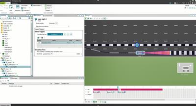
Figure 1: AVL Scenario Designer
Scenario Simulation Platform powered by Model.CONNECT
Virtualization of testing is the only viable solution for massive scaling and to manage the resulting testing effort. We now take this one step further by providing a platform that allows you to test your ADAS/AD software stack modules separately in multiple simulation environments. By choosing the adequate model and tool fidelity based on the system under test, costs can be significantly optimized.
Deploy your workloads on local machines or short-term rented virtual clusters in the cloud with our flexible job management system. You can also easily automate your integration and simulation tasks using our powerful Python API.
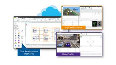
Figure 2: Scenario simulation platform powered by Model.CONNECT
Updates and improvements to AVL's simulation solution
Don't miss the latest enhancements in the area of Virtual System Development.
Dynamic E-Machine: Internal Inverter and Three-Phase Model
The Dynamic E-Machine component has been extended to enable inverter behavior to be modelled. The inverter model type is described either as an average voltage source converter or as a pulse-width modulation (PWM) voltage source converter.
The PWM approach offers the advantage that the component can be controlled by PWM signals. In this case, the internal inverter allows the application of an e-machine model operating on three phases. The simulation results show three-phase details including switching current and voltage in the different branches of the inverter and in the corresponding branches of the e-machine.
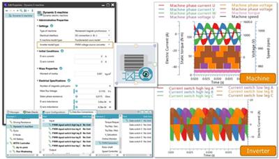
Figure 1: Three-phase dynamic e-machine and inverter
Powertrain Model Generator: Standard Reports
Extension of the Powertrain Model Generator to provide automatically generated result pages.
The scope of the result pages depends on the powertrain configuration selected and the results include time resolved data and scalar KPIs. The standard reports facilitate the assessment of powertrain configurations by providing a focused summary for review.
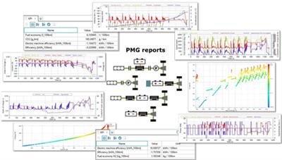
Figure 2: Powertrain Model Generator (PMG) standard reports
nD Map: Handling of Higher Dimensional Data
When physical modeling reaches its limits or when comprehensive experimental data are available, an effective dealing with multidimensional data comes into the spotlight. To this end, CRUISE M introduces a new dedicated nD Map component.
Data is stored in tabular form and is individually configurable. You can divide the columns into any number of domains and co-domains, the former requires inputs and the latter the outputs of the data evaluations. Corresponding data bus input and output ports are created automatically. This allows maps (i.e. loss as function of speed and torque) to be placed under other maps (i.e. gear and temperature), thus dividing a higher dimensional data structure (i.e. 5D) into smaller entities. Data assessment is thus made much easier.
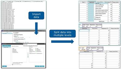
Figure 3: Multi-dimensional data handling with new nD Map
Result Storage: MAT Files Support
CRUISE M simulation results can be saved as ASCII files (i.e., CVS) and in binary format. Now another option has been added and results can also be saved in MAT file format.
Results saved as MAT files can naturally be used for standard post-processing in AVL IMPRESS™ M. In addition, they can be loaded into MATLAB®. The result data itself is delivered in a structured form. Global metadata and the list of components are on the top level. From there, you can drill down to the level of individual signals and perform any type of result analysis.
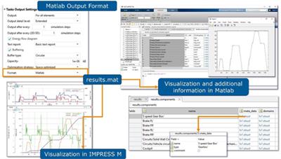
Figure 4: New result output as MAT file enables additional results assessment options
Discretized Solid 3D: Thermal Propagation
The propagation of heat through a 3D structure can be easily studied with the new functionality of the Discretized Solid 3D component.
On the new input page, you specify the layers where heat is to be released. Despite the simplicity of the input, you can accurately view the effect of a local temperature increase on neighboring zones. In addition, you can analyze the propagation of a temperature wave through the entire solid structure.
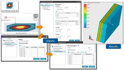
Figure 5: 3D simulation results using the internal heat source
Gear Box: Dynamic Shifting Model
Dynamic switching models are often the better choice for (virtual) test bed applications.
A kinematic shifting model describes the shifting process exactly in time and requires sophisticated numerical treatment in the background. The dynamic shift model avoids exactly that. Therefore, we have now extended the Gear Box component and the existing kinematic-fixed shifting process with the possibility to describe the shifting process dynamically.
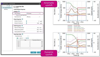
Figure 6: Gear Box dynamic shifting model
Updates and improvements to AVL's simulation solution
At a glance: The highlights of the simulation solutions in the area of Virtual ICE Development Performance and Emissions.
New Engine Segment Modeler Available in AVL FIRE M
We are proud to offer you an ESE Diesel Successor in AVL FIRE™ M - very easy to use, fast to set up and execute.
When developing this feature, particular attention was paid to making the setup process of the fully automated segment mesh generation as simple as possible. This significantly reduces the overall complexity of the modeling process, which in turn makes it easy for less experienced users to get started with segment CFD simulations for combustion engines.
The new feature combines the proven tools AVL FAME M Engine and AVL FAME Poly. It is integrated in the AVL Simulation Desktop and is called AVL FAME M Engine S.
The only mandatory inputs required to start the FAME M Engine S process are 2D curves describing the piston geometry and the crank train dimensions. Optionally, you can add a parameterized nozzle tip contour. Furthermore, blow-by and compensation volumes can be activated and will be added automatically to the mesh. FAME M Engine S uses this information to intelligently find the optimal mesh settings for the specified geometry and performs its generation, fully automatically. All required selections are automatically created with this input.
The resulting meshes are polyhedral meshes (consistent with FAME M Engine and the Port Workflow) with identical node distribution on the cyclic boundaries.
They contain local refinements for spray jets and similar features. All FAME M Engine S inputs can be provided as parameters, making it easier than ever to perform case studies.
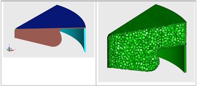
Figure 1: Surface data with automatically defined selections (left) and computational polyhedral-cell-grid including details such as nozzle tip and piston/liner clearance as well as perfect grid boundary layers (right).
Engine Thermodynamics Highlights in AVL CRUISE M
-Multi-Entry Turbine:The turbine component is extended to handle multiple entries and their impact on the turbine
-Restriction / Throttle:This release of AVL CRUISE M enables you to model pressure recovery effects in the restriction and throttle components.
-Engine Parameterization Wizard (EPW):The Wizard has been enhanced with new functionality und improved usability
-Gas Dynamic Pipe:The robustness and efficiency of 1D gas dynamics simulations have been improved by introducing a new method to describe momentum conservation at the inlet and outlet face of a pipe.
-Quasi-Propagatory Gas Dynamics Model (QPM):the Quasi-Propagatory Model (QPM) fills the gap between lumped-parameter models and distributed-parameter models, allowing the simulation of propagation effects, even in a compact, lumped parameter framework
-Engineering Enhanced Diesel Cylinder:New models to describe the delivery ratio, the concentration of the residual gas and friction loses have been introduced. The parameterization wizard, which comes with the cylinder model, has been improved to simplify the parameterization of NOx emissions, delivery ratio and the friction model.
Exhaust Gas Aftertreatment Highlights in AVL CRUISE M
-Parameter Masking:This release renders additional User Coding Interface (UCI) parameters from various filter and catalyst input pages applicable to the masking technology
Highlights AVL FIRE M IC Engine Performance and Emissions
-New multi-component flash boiling model:FIRE M R2022.2 offers a flash boiling model that is applicable to multi-component fuels.
This is of particular interest with respect to up-coming emission regulations. Simulation engineers who enhance their models by including multi-component surrogate fuels for spray and engine combustion can now improve accuracy and predictivity. The model addresses various physical processes like fuel nozzle tip wetting, spray plume-plume interaction, spray collapse due to sudden depressurization and other processes, all of which affect engine performance, efficiency and formation of emissions.
-Lagrangian spray now available for Embedded Body-Models:The models related to Lagrangian spray calculations are now able to account for static or moving embedded surfaces within the finite volume computational grid.
-SCR App:This release contains a new solution app for SCR / AdBlue injection simulation as a beta version. The app allows you to define FIRE M single and multi-domain models for standard SCR simulations following the defaults that are also available in the FIRE M SCR templates. It supports both steady state pre-calculation as well as steady state and transient SCR simulation with the standard SCR thermolysis or detailed decomposition model. In addition, the spray nozzle setup, coupled thin wall model, and porosity settings can be used.
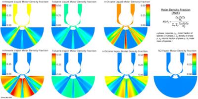
Figure 2: Multi-component flash boiling: Molar density fraction of liquid and vapor phase species at 0.4 ms after start of injection
Updates and improvements to AVL's simulation solution
PEMFC and SOxC Stacks in 3D
The 3D stack model has set a milestone on the system level. The three-dimensional representation allows you to study the impact of spatial non-uniformities on stack performance characteristics without having to perform extensive CFD simulations.
The PEM Fuel Cell (PEMFC) models and the Solid Oxide Fuel Cell and Electrolyzer (SOxC) components in CRUISE M have been extended to fully reflect the stack behavior in 3D. You can configure spatial resolution in all three dimensions: Select between straight or serpentine gas channels and choose between parallel or crossflow as the flow type. Non-uniform inlet flow conditions are handled using dedicated input maps covering the two dimensions of the cathode and anode inlet face, respectively. The thermal 3D stack model can be connected to CRUISE M's liquid and gas networks in a freely configurable way to describe any kind of stack thermoregulation. Result analysis is supported by full 3D postprocessing, by dedicated 2D cuts, and by time-based data at user-defined measurement positions.
The measured CPU times for representative model sizes, i.e. number of segments used for spatial discretization, show real-time factors in the range between 0.25 (50 segments) to 3 (600 segments).
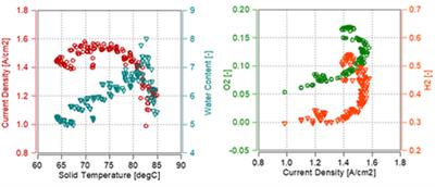
Figure 1: The 3D stack model in AVL CRUISE M provides information regarding local states for individual cells in the stack relevant for performance, degradation and cold start
PEM Fuel Cell Ready-to-Run Models
The PEM Fuel Cell Model (PEMFC) Generator, first released in CRUISE M 2022R1, has been extended to support the parameterization of the stack model based on measurement data with the help of built-in optimization techniques. In this version of CRUISE M, not only the stack component is automatically generated but also all the infrastructure components needed to run the model. This involves a closed electrical circuit, gas networks for the anode and cathode supply, control functions to operate the plant, the measurement data used for the parameterization and tailored dashboards for online monitoring and result postprocessing. At the end of this process, a stack component model is available for further use featuring the optimized model parameters representing the reference data with highest accuracy. Having gone through the Fuel Cell Model Generator, you need to do nothing more than click "Run".
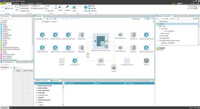
Figure 2: Ready-to-run model topology displayed in the AVL CRUISE™ M Graphical User Interface
Evaporator Model for SOFC Systems
When operating Solid Oxide Fuel Cell (SOFC) systems with liquid fuels such as methanol and ethanol, the fuels must be vaporized before being supplied to the SOFC stack. The evaporation and condensation of liquid species into and from a gas phase is now supported by CRUISE M.
You can now choose between the five gas path components: Plenum, Quasi Dimensional Pipe, Restriction, Gas Heat Exchanger and Gas Flow Loss. Optionally, CRUISE M offers the possibility to configure a dedicated liquid film that interacts with the gas flow. The film model takes into account convective heat exchange with the gas, conductive heat transfer to the underlying wall, and the latent heat consumed/released during evaporation/condensation. All required liquid properties are provided by the property database. The film mass may additionally change due to trapping of liquid droplets from the gas stream or release of droplets due to the carry away effects. Heat transfers and evaporation/condensation follow fundamental physical considerations that are influenced by the selected liquid properties and flow conditions. It is worth mentioning that trapping and carry away effects are modeled in an empirical way.
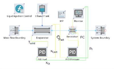
Figure 3: Schematics of evaporator component model integration into an AVL CRUISE M SOFC system model
There have also been new developments related to AVL FIRE M.
Platinum Band Formation Model
The existing PEM Fuel Cell Degradation Models in our CFD tool AVL FIRE™ M have been extended with an additional chemical degradation effect. This release of FIRE M allows you to simulate the formation of a platinum band in the polymer electrolyte membrane. The formation of the Pt band is actually the result of an undesirable effect, namely the loss of Pt in the catalyst layer of the cathode. However, the band formation also has a positive effect. The consumption of hydrogen in the membrane by the platinum band protects the cathode catalyst layer from a larger amount of hydrogen cross-over, thus reducing the effects of parasitic reactions.
In detail, the platinum ions generated in the cathode catalyst layer by dissolution of the metallic platinum diffuse into the membrane, where they react with crossover hydrogen coming from the anode to form solid platinum crystallite. This leads to the formation of a catalytic surface inside the membrane called a platinum band. The location and size of the platinum band is determined by local operating conditions such as temperature, potential or concentrations. Beside the reaction between platinum ions and hydrogen, additional reactions occur at the new catalyst surface, for example oxygen and hydrogen reduction, hydrogen peroxide reduction and Pt-dissolution.
Combined with the existing catalyst layer and membrane degradation models available in FIRE M, you can analyze in spatial and temporal details the reduction of the electrochemically active surface area (ECSA) that leads to a loss of fuel cell performance over time. Thanks to the unique numerical methods in FIRE M, you can efficiently simulate, for example, the impact of multiple voltage cycles of accelerated-stress-tests, covering several hundred hours of operation, on the performance evolution of the PEM fuel cell.
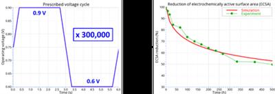
Figure 4: Reduction of electrochemically active surface area (ECSA) in simulation and experiment during 300.000 trapezoidal voltage cycles between 0.9V and 0.6V
Electrochemical Hydrogen Compressor Model
The Fuel Cell Module in FIRE M now offers you a model for the simulation of low-temperature PEM hydrogen compressors.
In an electrochemical hydrogen compressor (EHC), hydrogen is continuously produced by supplying electrical energy in a closed system. The process runs until the desired pressure, max. up to 700 bar, is reached. Compared to conventional mechanical hydrogen compression, an EHC has a number of advantages. These include higher efficiency, noiseless operation and robustness.
Design: The EHC is a combination of a PEM electrolyzer and a PEM fuel cell. Like the PEM fuel cell, hydrogen is oxidized at the anode side, producing hydrogen protons and electrons, and similar to a PEM electrolyzer, hydrogen is produced at the cathode side by recombining hydrogen protons and electrons. The materials of an EHC are basically the same as for a PEM fuel cell.
You can use the new EHC model in both transient and steady run mode. You will gain insights into the mass and heat transport and electrochemical processes, allowing you to determine the impact of hardware design features, membrane and GDL material properties, and operating conditions on performance and efficiency.
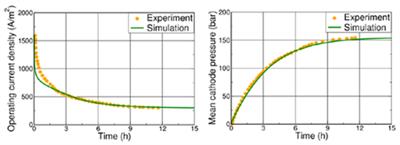
Figure 5: Comparison of simulated current density and pressure build-up with experimental data from literature for an
Electrochemical Hydrogen Compressor (EHC) cell
Simulation has long been a core AVL competence,and our Advanced Simulation Technologies (AST) business unit has solutions for a multitude of applications. They offer high-definition insights into the behavior and interactions of components, systems and entire vehicles. Our simulation solutions drive automotive efficiency, performance and innovation, while reducing development effort, costs and time-to-market. Used on their own, or combined with other methodologies and third-party tools, they support OEMs in the creation of market-leading products that meet global legislation.
AVL CRUISE / AVL CRUISE M
With more than 11,000 employees, AVL is the world's largest independent companyfor development, simulation and testing in the automotive industry, and in other sectors. Drawing on its pioneering spirit, the company provides concepts, solutions and methodologies to shape future mobility trends. AVL creates innovative and affordable technologies to effectively reduce CO2 by applying a multi-energy carrier strategy for all applications - from hybrid to battery electric and fuel cell technologies. The company supports customers throughout the entire development process from the ideation phase to serial production. To accelerate the vision of smart and connected mobility AVL has established competencies in the fields of ADAS, autonomous driving and digitalization.
AVL's passion is innovation. Together with an international network of experts that extends over 26 countries and with 45 Tech- and Engineering Centers worldwide, AVL drives sustainable mobility trends for a greener future. In 2020, the company generated a turnover of 1.7 billion Euros, of which 12% are invested in R&D activities.
Download From 1DL
https://1dl.net/0y7a5bka7h5f/rlpsm.AVL.Simulation.Suite.2022.R2.part01.rar.html
https://1dl.net/trtk0fwugx23/rlpsm.AVL.Simulation.Suite.2022.R2.part02.rar.html
https://1dl.net/mk89mz8a3l4s/rlpsm.AVL.Simulation.Suite.2022.R2.part03.rar.html
https://1dl.net/kj1l9u376q5o/rlpsm.AVL.Simulation.Suite.2022.R2.part04.rar.html
https://1dl.net/byx67nzynvq3/rlpsm.AVL.Simulation.Suite.2022.R2.part05.rar.html
https://1dl.net/krety1odn5ln/rlpsm.AVL.Simulation.Suite.2022.R2.part06.rar.html
https://1dl.net/x7tlvq5f8dz6/rlpsm.AVL.Simulation.Suite.2022.R2.part07.rar.html
https://1dl.net/cu7e6k4gdodj/rlpsm.AVL.Simulation.Suite.2022.R2.part08.rar.html
https://1dl.net/hnlzxz2d5b24/rlpsm.AVL.Simulation.Suite.2022.R2.part09.rar.html
https://1dl.net/1f47u308b8eo/rlpsm.AVL.Simulation.Suite.2022.R2.part10.rar.html

https://uploadgig.com/file/download/f9Cef92715d944d4/rlpsm.AVL.Simulation.Suite.2022.R2.part01.rar
https://uploadgig.com/file/download/a91e744F3ae623f3/rlpsm.AVL.Simulation.Suite.2022.R2.part02.rar
https://uploadgig.com/file/download/7A74F3f6359f8bc0/rlpsm.AVL.Simulation.Suite.2022.R2.part03.rar
https://uploadgig.com/file/download/aEDF9a1ee63b95e1/rlpsm.AVL.Simulation.Suite.2022.R2.part04.rar
https://uploadgig.com/file/download/f94797fEE3Df3b4f/rlpsm.AVL.Simulation.Suite.2022.R2.part05.rar
https://uploadgig.com/file/download/547cdc3f33084641/rlpsm.AVL.Simulation.Suite.2022.R2.part06.rar
https://uploadgig.com/file/download/8faa074Ddb4949b6/rlpsm.AVL.Simulation.Suite.2022.R2.part07.rar
https://uploadgig.com/file/download/2c23cb673ddBF337/rlpsm.AVL.Simulation.Suite.2022.R2.part08.rar
https://uploadgig.com/file/download/127cd6bE81cC5c6d/rlpsm.AVL.Simulation.Suite.2022.R2.part09.rar
https://uploadgig.com/file/download/c0729d1a13877349/rlpsm.AVL.Simulation.Suite.2022.R2.part10.rar

https://rapidgator.net/file/adcb06ef48388e6848fc4af87930df99/rlpsm.AVL.Simulation.Suite.2022.R2.part01.rar.html
https://rapidgator.net/file/cdf9413c566d4f3239be31860495fa7c/rlpsm.AVL.Simulation.Suite.2022.R2.part02.rar.html
https://rapidgator.net/file/e1ec92b8f805c679c5bc707d76008104/rlpsm.AVL.Simulation.Suite.2022.R2.part03.rar.html
https://rapidgator.net/file/c958837c882bd809277e6b6aca973c87/rlpsm.AVL.Simulation.Suite.2022.R2.part04.rar.html
https://rapidgator.net/file/1b04542474a4041bde98a714949a161e/rlpsm.AVL.Simulation.Suite.2022.R2.part05.rar.html
https://rapidgator.net/file/2946baf365f2e07a096c598c296dde1d/rlpsm.AVL.Simulation.Suite.2022.R2.part06.rar.html
https://rapidgator.net/file/4a3f2890b1403151e9803a16748e835a/rlpsm.AVL.Simulation.Suite.2022.R2.part07.rar.html
https://rapidgator.net/file/ce0d57f765d4eb32105fb70d6cc42dd3/rlpsm.AVL.Simulation.Suite.2022.R2.part08.rar.html
https://rapidgator.net/file/afd3e6f51e7711f7c240d6f5132819d1/rlpsm.AVL.Simulation.Suite.2022.R2.part09.rar.html
https://rapidgator.net/file/ac7b10e81790f06d0bb09abddc3c3591/rlpsm.AVL.Simulation.Suite.2022.R2.part10.rar.html

https://nitroflare.com/view/3BC037A344DDBC7/rlpsm.AVL.Simulation.Suite.2022.R2.part01.rar
https://nitroflare.com/view/953E29AD9F9880A/rlpsm.AVL.Simulation.Suite.2022.R2.part02.rar
https://nitroflare.com/view/2AD7C3E896611BC/rlpsm.AVL.Simulation.Suite.2022.R2.part03.rar
https://nitroflare.com/view/51AC38A58017131/rlpsm.AVL.Simulation.Suite.2022.R2.part04.rar
https://nitroflare.com/view/A05F63B13DE7D20/rlpsm.AVL.Simulation.Suite.2022.R2.part05.rar
https://nitroflare.com/view/F9EC06D103D6D7B/rlpsm.AVL.Simulation.Suite.2022.R2.part06.rar
https://nitroflare.com/view/965BCAA945FDEC7/rlpsm.AVL.Simulation.Suite.2022.R2.part07.rar
https://nitroflare.com/view/CE0903F34B8B4DA/rlpsm.AVL.Simulation.Suite.2022.R2.part08.rar
https://nitroflare.com/view/F6B12AFA35EB8F4/rlpsm.AVL.Simulation.Suite.2022.R2.part09.rar
https://nitroflare.com/view/125AFF46921995B/rlpsm.AVL.Simulation.Suite.2022.R2.part10.rar
https://1dl.net/0y7a5bka7h5f/rlpsm.AVL.Simulation.Suite.2022.R2.part01.rar.html
https://1dl.net/trtk0fwugx23/rlpsm.AVL.Simulation.Suite.2022.R2.part02.rar.html
https://1dl.net/mk89mz8a3l4s/rlpsm.AVL.Simulation.Suite.2022.R2.part03.rar.html
https://1dl.net/kj1l9u376q5o/rlpsm.AVL.Simulation.Suite.2022.R2.part04.rar.html
https://1dl.net/byx67nzynvq3/rlpsm.AVL.Simulation.Suite.2022.R2.part05.rar.html
https://1dl.net/krety1odn5ln/rlpsm.AVL.Simulation.Suite.2022.R2.part06.rar.html
https://1dl.net/x7tlvq5f8dz6/rlpsm.AVL.Simulation.Suite.2022.R2.part07.rar.html
https://1dl.net/cu7e6k4gdodj/rlpsm.AVL.Simulation.Suite.2022.R2.part08.rar.html
https://1dl.net/hnlzxz2d5b24/rlpsm.AVL.Simulation.Suite.2022.R2.part09.rar.html
https://1dl.net/1f47u308b8eo/rlpsm.AVL.Simulation.Suite.2022.R2.part10.rar.html

https://uploadgig.com/file/download/f9Cef92715d944d4/rlpsm.AVL.Simulation.Suite.2022.R2.part01.rar
https://uploadgig.com/file/download/a91e744F3ae623f3/rlpsm.AVL.Simulation.Suite.2022.R2.part02.rar
https://uploadgig.com/file/download/7A74F3f6359f8bc0/rlpsm.AVL.Simulation.Suite.2022.R2.part03.rar
https://uploadgig.com/file/download/aEDF9a1ee63b95e1/rlpsm.AVL.Simulation.Suite.2022.R2.part04.rar
https://uploadgig.com/file/download/f94797fEE3Df3b4f/rlpsm.AVL.Simulation.Suite.2022.R2.part05.rar
https://uploadgig.com/file/download/547cdc3f33084641/rlpsm.AVL.Simulation.Suite.2022.R2.part06.rar
https://uploadgig.com/file/download/8faa074Ddb4949b6/rlpsm.AVL.Simulation.Suite.2022.R2.part07.rar
https://uploadgig.com/file/download/2c23cb673ddBF337/rlpsm.AVL.Simulation.Suite.2022.R2.part08.rar
https://uploadgig.com/file/download/127cd6bE81cC5c6d/rlpsm.AVL.Simulation.Suite.2022.R2.part09.rar
https://uploadgig.com/file/download/c0729d1a13877349/rlpsm.AVL.Simulation.Suite.2022.R2.part10.rar

https://rapidgator.net/file/adcb06ef48388e6848fc4af87930df99/rlpsm.AVL.Simulation.Suite.2022.R2.part01.rar.html
https://rapidgator.net/file/cdf9413c566d4f3239be31860495fa7c/rlpsm.AVL.Simulation.Suite.2022.R2.part02.rar.html
https://rapidgator.net/file/e1ec92b8f805c679c5bc707d76008104/rlpsm.AVL.Simulation.Suite.2022.R2.part03.rar.html
https://rapidgator.net/file/c958837c882bd809277e6b6aca973c87/rlpsm.AVL.Simulation.Suite.2022.R2.part04.rar.html
https://rapidgator.net/file/1b04542474a4041bde98a714949a161e/rlpsm.AVL.Simulation.Suite.2022.R2.part05.rar.html
https://rapidgator.net/file/2946baf365f2e07a096c598c296dde1d/rlpsm.AVL.Simulation.Suite.2022.R2.part06.rar.html
https://rapidgator.net/file/4a3f2890b1403151e9803a16748e835a/rlpsm.AVL.Simulation.Suite.2022.R2.part07.rar.html
https://rapidgator.net/file/ce0d57f765d4eb32105fb70d6cc42dd3/rlpsm.AVL.Simulation.Suite.2022.R2.part08.rar.html
https://rapidgator.net/file/afd3e6f51e7711f7c240d6f5132819d1/rlpsm.AVL.Simulation.Suite.2022.R2.part09.rar.html
https://rapidgator.net/file/ac7b10e81790f06d0bb09abddc3c3591/rlpsm.AVL.Simulation.Suite.2022.R2.part10.rar.html

https://nitroflare.com/view/3BC037A344DDBC7/rlpsm.AVL.Simulation.Suite.2022.R2.part01.rar
https://nitroflare.com/view/953E29AD9F9880A/rlpsm.AVL.Simulation.Suite.2022.R2.part02.rar
https://nitroflare.com/view/2AD7C3E896611BC/rlpsm.AVL.Simulation.Suite.2022.R2.part03.rar
https://nitroflare.com/view/51AC38A58017131/rlpsm.AVL.Simulation.Suite.2022.R2.part04.rar
https://nitroflare.com/view/A05F63B13DE7D20/rlpsm.AVL.Simulation.Suite.2022.R2.part05.rar
https://nitroflare.com/view/F9EC06D103D6D7B/rlpsm.AVL.Simulation.Suite.2022.R2.part06.rar
https://nitroflare.com/view/965BCAA945FDEC7/rlpsm.AVL.Simulation.Suite.2022.R2.part07.rar
https://nitroflare.com/view/CE0903F34B8B4DA/rlpsm.AVL.Simulation.Suite.2022.R2.part08.rar
https://nitroflare.com/view/F6B12AFA35EB8F4/rlpsm.AVL.Simulation.Suite.2022.R2.part09.rar
https://nitroflare.com/view/125AFF46921995B/rlpsm.AVL.Simulation.Suite.2022.R2.part10.rar
Links are Interchangeable - No Password - Single Extraction
